7.6 Model tuning
After identifying promising models in the previous step the next step is to optimize the hyperparameters of the model to achieve better predictive performance. Depending on the model there can be many hyperparameters. hyperparameters define specifics of the model, e.g. the number of trees for random forests. To find the optimum combination of hyperparameters optimization algorithms like genetic algorithms can be utilized.
Model tuning: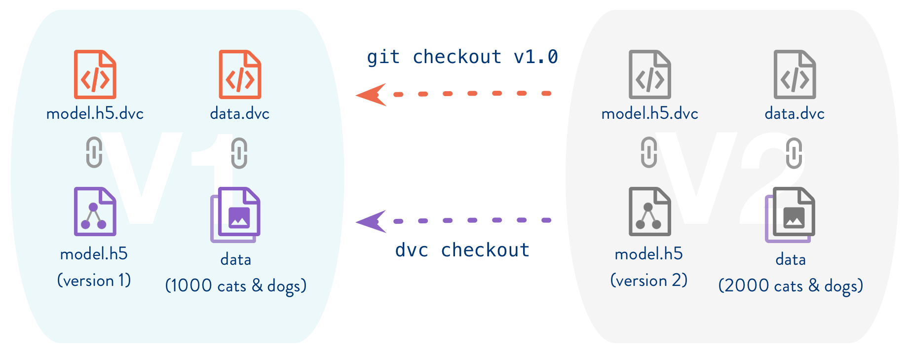
- Find best combination of hyperparameters
- number of trees for random forest
- learning rate for neural networks
- Optimizing algorithms can be utilized
- genetic algorithms
- simulated annealing
- Manage models and results
- use tool such as DVC https://dvc.org
- Open-source Version Control System for ML Projects
- use tool such as DVC https://dvc.org
There are may different metrics for which the model can be optimized
7.6.1 Metrics
Metrics express how well suited a model is for a given task. Depending on what is needed from the model different metrics can be employed. For classification and regression models different metrics are defined.
7.6.1.1 Metrics for classification
Metrics for classification express how well the model assigns classes to the samples
Accuracy
Is the ratio of correct predictions to total number of predictions for classification problems. For unbalanced data sets the accuracy is not very well suited
Accuracy:
- Ratio of correct to total predictions
- Not suited for unbalanced data set
- Two class problem
- 98% class A, 2% class B
- Predict always class A
- \(\implies\) accuracy = 98%
\(\text{Accuracy} = \frac{\text{Number of Correct predictions}}{\text{Total number of predictions made}}\)
Log Loss
Logarithmic Loss or Log Loss becomes high if a sample is misclassified and therefore penalizes them.
Logarithmic Loss: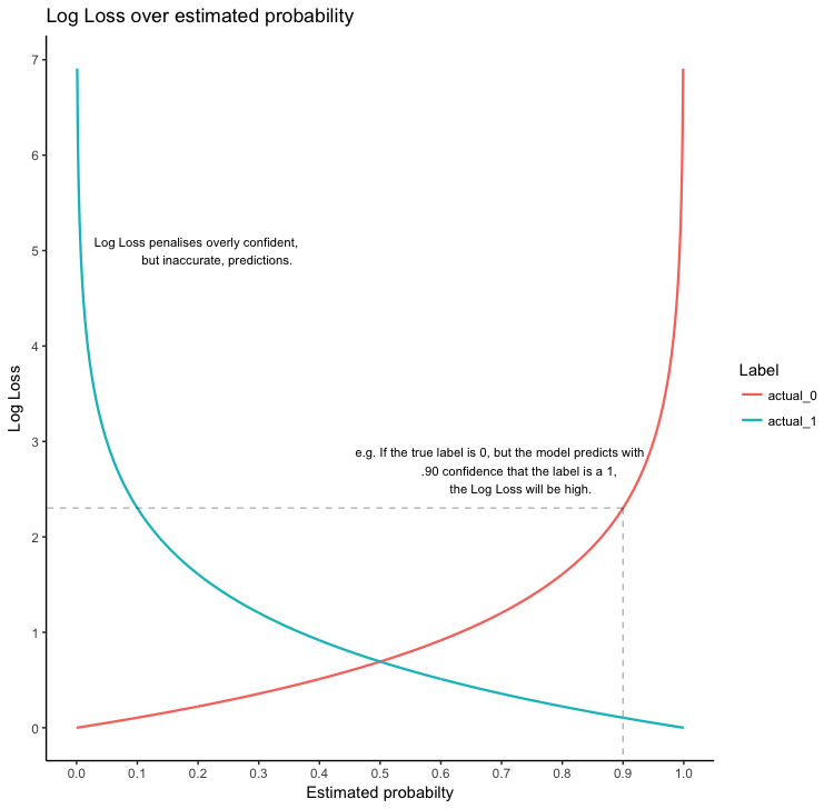
- penalizes misclassifications
- log loss near 0 \(\implies\) accuracy \(\Uparrow\)
\[\text{Logarithmic Loss}=\frac{-1}{N} \sum_{i=1}^{N} \sum_{j=1}^{M} y_{i j} * \log \left(p_{i j}\right)\]
where:
- \(y_{i j}\): indicates whether sample \(i\) belongs to class \(j\) or not
- \(p_{i j}\): indicates probability of sample \(i\) belongs to class \(j\)
7.6.1.1.1 Receiver operating characteristic (ROC)
The result of a classification with two classes (binary classification) is given as a percentage value of how sure the algorithm is that the sample belongs to a class. Depending on the the overall project target the threshold upon which the class is rated as identified is set. If a false positive is to be avoided than the threshold for classifying a positive is set high.
ROC is a graphical representation of how the chosen threshold affects the specificity and sensitivity of the model.
Receiver operating characteristic (ROC):
- Result of classification is probability of belonging to class
- Thresholds divides classes
- Selection of threshold changes
- sensitivity
- specificity
- ROC is graphical representation of threshold variation
A detailed explanation is given in chapter 25.4.2
Area under curve (AUC)
The area under the Receiver operating characteristic (ROC) curve is called AUC. Since it is a numerical value it is suited to act as a metric to optimize a model. The value is in the range of \(0\leq AUC \geq 1\), the better the algorithm predicts the classes the higher the value. If all samples are predicted correctly the AUC = 1
Area under curve (AUC):
- Numeric value
- can be used to optimize hyperparameters
- Value range \(0\leq AUC \geq 1\)
- The better the model the higher AUC perfect model \(\implies\) AUC = 1
Confusion matrix
Confusion matrix is a matrix which contains the number of all combinations of predicted and true labels. It is a powerful metric but needs some practice to read.
Confusion matrix: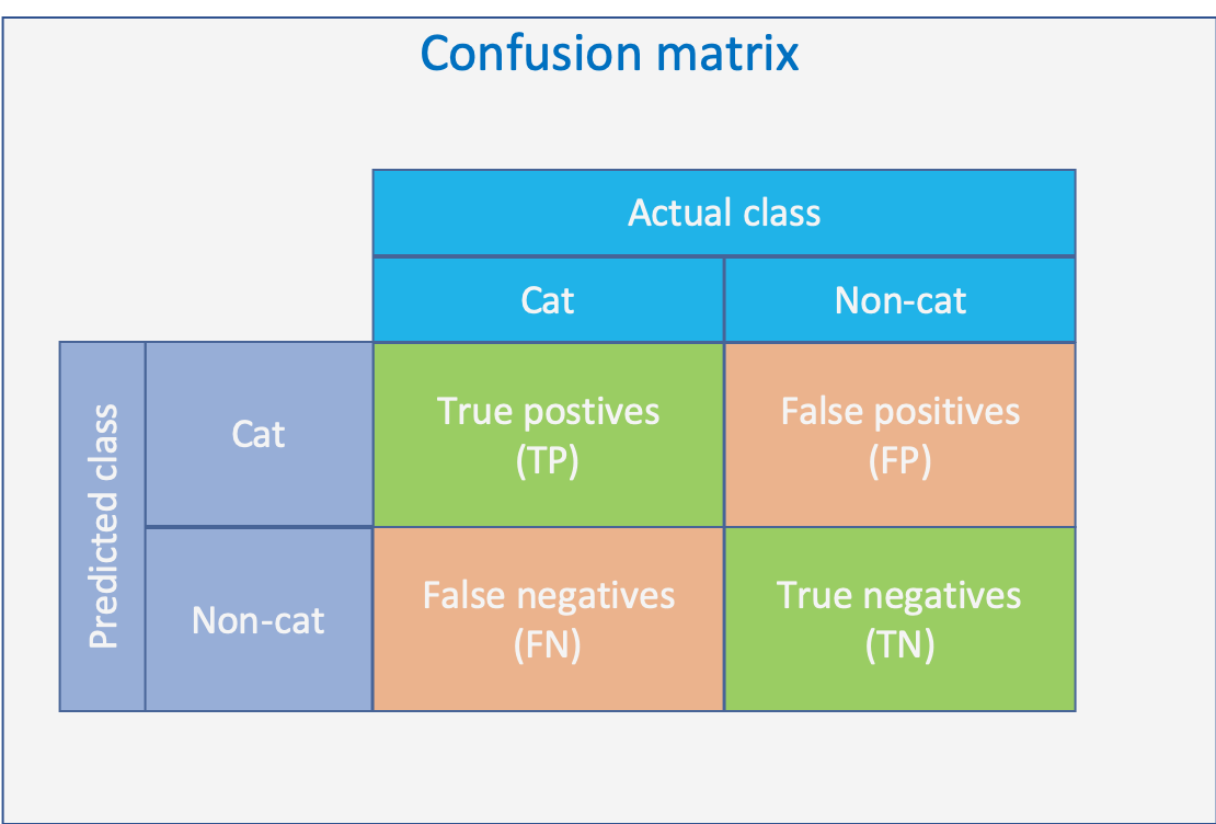
- Matrix of all combinations of predicted and true labels
- true positives (TP)
- true negatives (TP)
- false positives (FP)
- false negatives (FN)
- All correct predictions are on diagonal of matrix
A detailed explanation is given in chapter 25.4
Precision
Precision is the ratio between correct positive predicted and all positive predicted samples
Precision \(=\frac{\text { True Positives }}{\text { True Positives }+\text { False Positives }}\)
Recall
Recall is the ratio between correct positive labels and all samples whit positive label. The metric is also called sensitivity
Recall \(=\frac{\text {True Positives}}{\text {True Positives }+\text { False Negatives}}\)
F1 score
The F1 score is a combination of precision and recall. The range is \(0\leq F1 \geq 1\) with better models have higher F1 scores.
F1 score: - Combining - precision - recall - Better models have higher value - value range \(0\leq F1 \geq 1\)
\[F 1=2 * \frac{1}{\frac{1}{\text { precision }}+\frac{1}{\text { recall }}}\]
Entropy
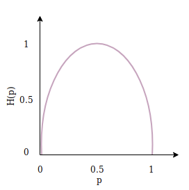
\(H(p, q)=-\sum_{x} p(x) \log q(x)\)
Softmax