3.9 Latent diffusion models (LDM)
With latent diffusion models a bunch of image generating related concepts can be implemented as described in (Rombach et al. 2022) and (Kawar et al. 2022).
LDM tasks:
- Image generation text2image
- Super resolution
- Inpainting
- Text-Based Real Image Editing
The graph depicting different conditioning of LDM in (Rombach et al. 2022) shows that there are different inference inputs to condition a LDM
LDM inference inputs:
- Semantic map
- Text
- Representations
- Images
Those inputs are used by simply concatenate them to the latent space variable or used via cröss-attention mechanism, well known from
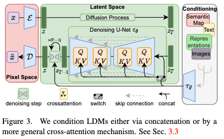
Conditioning of LDM, source: (Rombach et al. 2022)
The secrete of stable diffusion’s success is that the denoising process is performed in the lower dimensional latent space which makes is faster and less computational expensive than in pixel space. Sounds confusing?
In the following examples are given and if interested a shallow dive into the theory with links for deep dives 🤿 is given. Also, in chapter 3.3 of (Rombach et al. 2022) a thorough explanation of the conditioning process is presented.
3.9.1 Image generation from text with LDM (text2img)
Creating images based on a text prompt, i.e the model generates an image based on the text input called prompt. The concept of how to connect the text to the image is depicted below.

Matching text and image in latent space, source: https://openai.com/blog/clip/
The prompt is mapped to a latent space via a language model such that multiplication of the resulting latent space vector with the latent space vector of the image gives a high value, whereas a multiplication with other images gives a low value, i.e. \(I_x * T_x >I_{\neq x} * T_x\).
Examples of images for given text prompts are shown below.
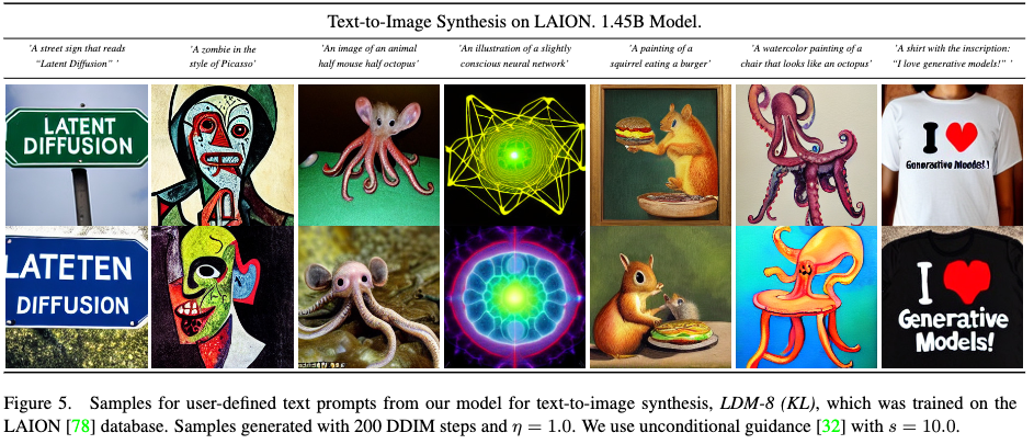
Image generation from text with LDM, source: (Rombach et al. 2022)
More examples of text2image can be found at lexica which is also a good place to discover how to phrase good prompts to achieve high quality images.
At the huggingface space one can experiment with those prompts, more info about the stable diffusion model of Stability AI can be found at Stable Diffusion v2 Model Card
3.9.2 Super resolution
LDMs can upscale the resolution of images as seen below.
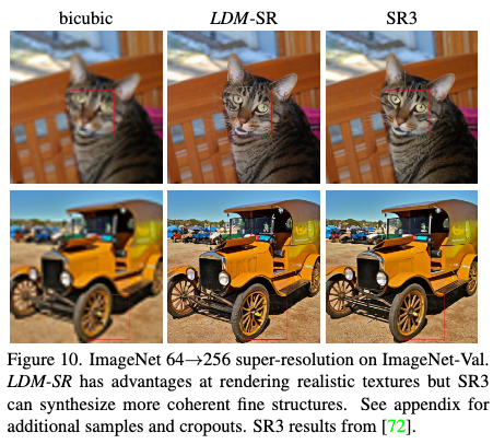
Super resolution with LDM, source: (Rombach et al. 2022)
3.9.3 Inpainting
Inpainting is the task of filling masked regions of an image with new content either because parts of the image are are corrupted or to replace existing but undesired content within the image.
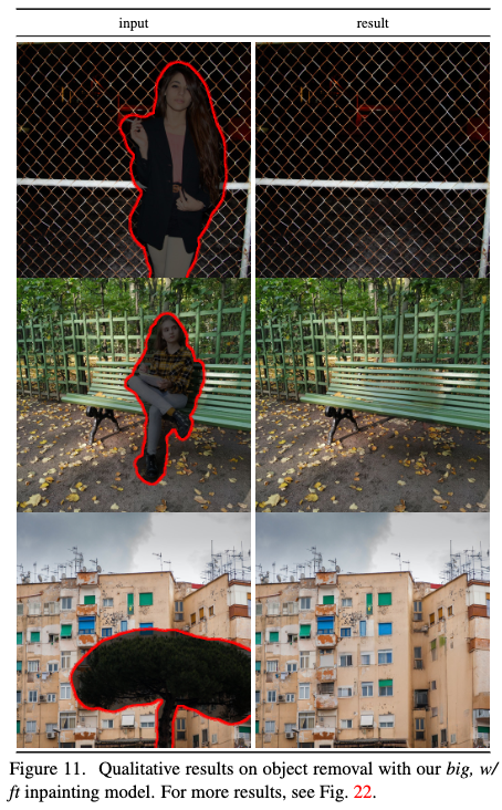
Inpainting with LDM, source: (Rombach et al. 2022)
3.9.4 Imagic: Text-Based Real Image Editing with Diffusion Models
Here the input is a text and an image, the output is an image where the input image is manipulated according to the input text.
Imagic inputs:
- Target text prompt
- Real image
Imagic steps:
- Encode target text => \(e_{tgt}\)
- Optimize \(e_{tgt}\) towards \(e_{opt}\) to reconstruct input image
- Fine tune generative model to improve fidelity to the input image, \(e_{opt}\) is fixed
- Interpolate between \(e_{tgt}\) and \(e_{opt}\) to generate resulting image
The schematic description is shown below.
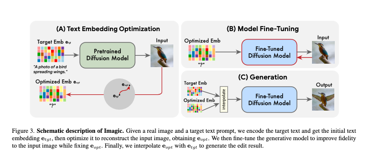
Schematic description of text-based real image editing with LDM, source: (Kawar et al. 2022)
Examples of edited images are shown below

Examples of text-based real image editing with LDM, source: (Kawar et al. 2022)
3.9.5 Stable diffusion under the hood
Great explanations of the algorithm are given at:
- Stable Diffusion with 🧨 Diffusers (Patil 2022)
- gives an code example and explains the concept along code which can be run in a Colab
- The Illustrated Stable Diffusion (Alammar 2022)
- explains the concept with great graphs and animations
3.9.5.1 How does Stable Diffusion work?
Here we will focus on the explanation given in (Patil 2022). Diffusion models can denoise random Gaussian noise step by step, i.e. they can produce images from a noise seed. This process can be guided by a text prompt. The three main components of the stable diffusion inference are:
Main components of stable diffusion inference:
- Autoendcoder (VAE)
- U-Net shaped neural network
- Text-encoder
3.9.5.1.1 Variational autoencoder (VAE)
An VAE is a U-shaped neural network consists of:
- encoder
- decoder
The encoder compresses the input to a lower dimensional space called latent space, the decoder reconstructs the input from the latent space. The image generation of stable diffusion is faster than previous concepts because it performs the denoising in the latent space and not in the higher dimensional pixel space.
During inference only the decoder of the VAE is needed.
The VAE aims at keeping similar inputs close together in the latent space which is essential for the generation of images from noise because similar values in the latent space will give similar images generated from the decoder. An example for the case of images of digits is given in Intuitively Understanding Variational Autoencoders
3.9.5.1.2 U-Net
The U-Net computes the noise residual of the latent space and, the residual is used to denoise the latent space image representation. This procedure is performed several times sequentially. The number of denoising steps can be reduced using by training neural networks to learn how to do several steps at once.
3.9.5.1.3 Text-encoder
The text-encoder transforms the input prompt text into embeddings which are meaningful for the U-Net. One model used is Openai’s CLIP model, described in CLIP: Connecting Text and Images.
3.9.5.2 Inference
The inference process is shown in the flow diagram below.
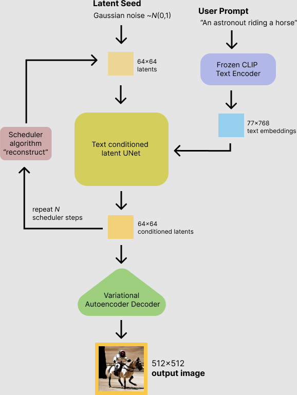
Stable diffusion inference, source: (Patil 2022)
A code example of the loop is given in the next section.
3.9.5.3 Code example for inference pipeline
A complete code example is given in (Patil 2022), the denoising loop is given below
from tqdm.auto import tqdm

scheduler.set_timesteps(num_inference_steps)

for t in tqdm(scheduler.timesteps):
    # expand the latents if we are doing classifier-free guidance to avoid doing two forward passes.
    latent_model_input = torch.cat([latents] * 2)

    latent_model_input = scheduler.scale_model_input(latent_model_input)

    # predict the noise residual
    with torch.no_grad():
        noise_pred = unet(latent_model_input, t, encoder_hidden_states=text_embeddings).sample

    # perform guidance
    noise_pred_uncond, noise_pred_text = noise_pred.chunk(2)
    noise_pred = noise_pred_uncond + guidance_scale * (noise_pred_text - noise_pred_uncond)

    # compute the previous noisy sample x_t -> x_t-1
    latents = scheduler.step(noise_pred, t, latents).prev_sample
The # perform guidance section shows how the prompt text is introduced in the inference step and how the guidance_scale controls the influence of the prompt text on the output.