9.5 Neural networks
non linear
activation
softmax types of layers siehe keras fully connected
9.5.1 Geometric Intuition for Training Neural Networks
The YouTube video by Leo Dirac gives are very intuitive explanation of how to a loss function is calculated in a 2-D example and also gives an introduction on Stochastic Weight Averaging (SWA). Leo also discusses minima in high dimensional space.
Stochastic Weight Averaging (SWA):
- Details at https://pytorch.org/blog/stochastic-weight-averaging-in-pytorch/
- High dimensional function have
- plenty of saddle points
- only one minima
- minima is wide
- train and test error surfaces are not perfectly aligned in the weight space
- therefore solution in middle of minima is better in terms of generalization
- what seems to be seperated minma are connected via one of the many dimensions
- SWA has been shown to significantly improve generalization in computer vision tasks
- SWA is shown to improve the stability of training as well as the final average rewards of policy-gradient methods in deep reinforcement learning
- SWA is suited for low precision training
Leo states his experience on twitter as follows:
Stochastic Weight Averaging (SWA) is totally magic! It takes me days to train my validation score down from 2.40 to 2.30, but just taking the mean of a bunch of checkpoints I have lying around and I'm down to 2.07. Thanks (andrewgwils?) and team for figuring this stuff out.
— Leo Dirac ((leopd?)) July 22, 2020
An implementation in PyTorch is shown below
from torchcontrib.optim import SWA

...
...

# training loop
base_opt = torch.optim.SGD(model.parameters(), lr=0.1)
opt = torchcontrib.optim.SWA(base_opt, swa_start=10, swa_freq=5, swa_lr=0.05)
for _ in range(100):
     opt.zero_grad()
     loss_fn(model(input), target).backward()
     opt.step()
opt.swap_swa_sgd()
9.5.2 Convolutional Neural Network (CNN) TBD
A Convolutional Neural Network is an neural network are mainly used to analyze image and audio data.
The following explanation is based on The learning machine tutorial “Classification Convolutional Neural Network (CNN)” https://www.thelearningmachine.ai/cnn
A classical CNN consists of
- one or more convolutoional layers
- one or more pooling layers
- one or more fully connected layers
A classical CNN is depicted in the image below
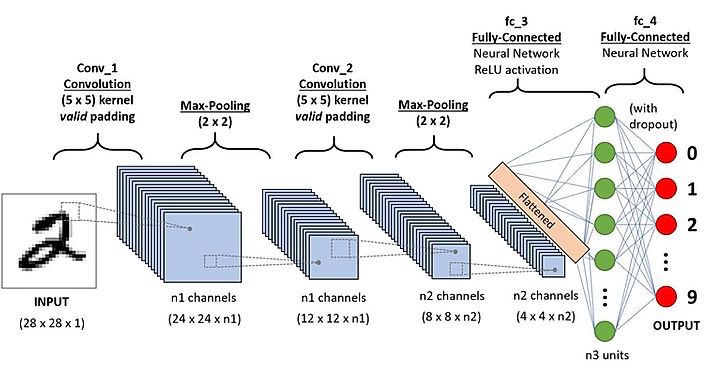
Figure from https://www.thelearningmachine.ai/cnn
An image is an 3 dimensional array where the third dimension are for the colors red, green and blue, in case of an RGB image. An image can therefore be represented as shown below
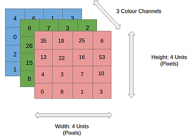
Figure from https://www.thelearningmachine.ai/cnn
To analyze an image the spatial relation between different pixels hold important information. Therefore it is beneficial to use an algorithm which looks not only at one pixel but also at the neighbouring pixels. One way of doing so is to slide an 2 dimensional array over the image array as can be seen below
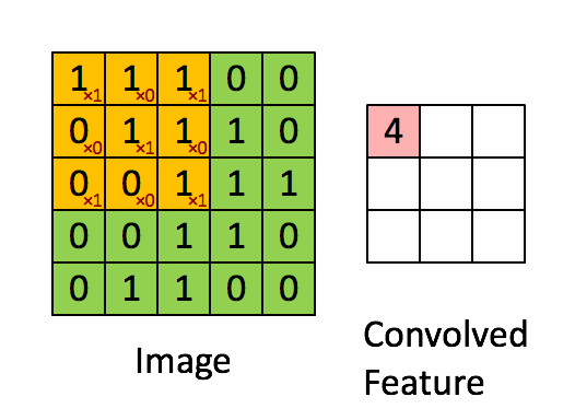
Figure from https://www.thelearningmachine.ai/cnn
The 2 dimensional array is called a kernel and is named depending on its dimensions. The kernel in the graph below is a “3 by 3 kernel”. Sliding the array across the image as gives a set of numbers as shown above. Those kernels can detect structures in images such as
- lines
- boxes
- circles
and kernels in later layers in the CNN can detect more complex structures such as
- faces
- wheels
- trees
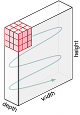
Figure from https://www.thelearningmachine.ai/cnn
A kernel has the same depth of the input, in a case of an RGB image, the depth of the kernel is 3. The output of the kernels is added, for each of the positions of the kernels there is one value at the output.
The movement across the image is based on the stride parameters for x and y direction. In the case below the stride is as follows
- stride x-direction = 1
- stride y-direction = 1
Depending on stride with and image dimension it might be necessary to apply padding, for details on padding see deepAi
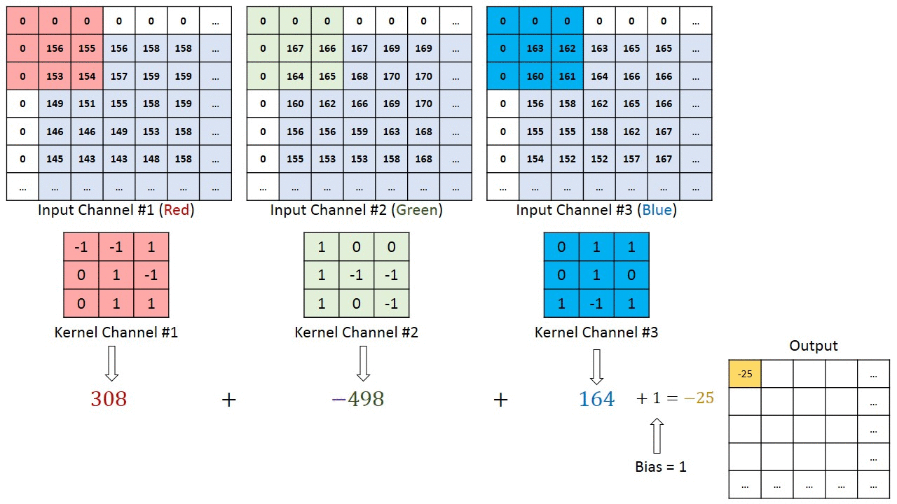
Figure from https://www.thelearningmachine.ai/cnn
9.5.2.1 Pooling layer
The pooling layer reduces the dimension as shown below. There are different types of pooling layers
- max
- average
below the working mechanism for a max pooling layer is shown. The stride for x and y is one, the dimension of the 5 by 5 input is reduced to 3 by 3
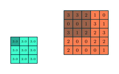
Figure from https://www.thelearningmachine.ai/cnn
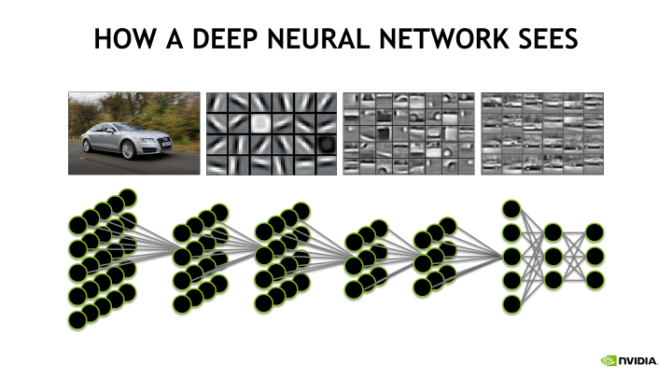
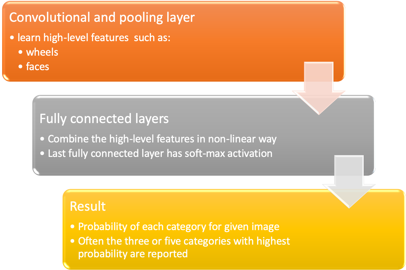
After one or more combination of convolutional and pooling layers one or more fully connected layers learn how to classify the image based on non-linear combinations of the high-level features learned by the previous layers.
 https://blogs.nvidia.com/wp-content/uploads/2018/09/autos-672x378.png
The fully connected layer with the soft-max activation at the end gives the probability of each category, often as a result the three to five classes with the highest probability are reported.
- convolutional and pooling layers => high-level features
- fully connected layers => combine non-linear high level features for classification
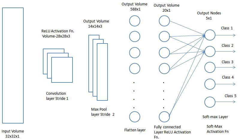
Figure from https://www.thelearningmachine.ai/cnn
The operating principle of a CNN is shown below
9.5.4 GANs
GANs from Scratch 1: A deep introduction. With code in PyTorch and TensorFlow
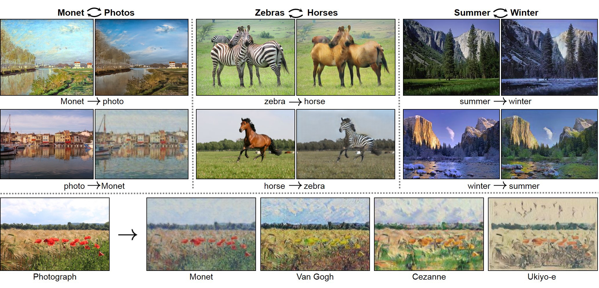
credit of the image (Zhu et al. 2017)
Generative models learn the intrinsic distribution function of the input data p(x) (or p(x,y) if there are multiple targets/classes in the dataset), allowing them to generate both synthetic inputs x’ and outputs/targets y’, typically given some hidden parameters.
GANs they have proven to be really succesfull in modeling and generating high dimensional data, which is why they’ve become so popular. Nevertheless they are not the only types of Generative Models, others include Variational Autoencoders (VAEs) and pixelCNN/pixelRNN and real NVP. Each model has its own tradeoffs.
Some of the most relevant GAN pros and cons for the are:
They currently generate the sharpest images
They are easy to train (since no statistical inference is required), and only back-propogation is needed to obtain gradients
GANs are difficult to optimize due to unstable training dynamics.
No statistical inference can be done with them (except here): GANs belong to the class of direct implicit density models; they model p(x) without explicitly defining the p.d.f.
A neural network G(z, θ₁)
Jupyter notebook on github https://github.com/diegoalejogm/gans/blob/master/1.%20Vanilla%20GAN%20PyTorch.ipynb