9.2 Logistic regression
Logistic regression is similar to linear regression, however, the value range of the dependent variable y is limited to: \(0\leq y \geq 1\)
Logistic regression is a algorithm with the low computational complexity
Logistic regression:
- Low computational complexity
- y limited range of values \(0\leq y \geq 1\)
- maps x on y (\(y \leftarrow x\)) using the logisit function
- Used of classification
The logistic function is depicted in the graph below
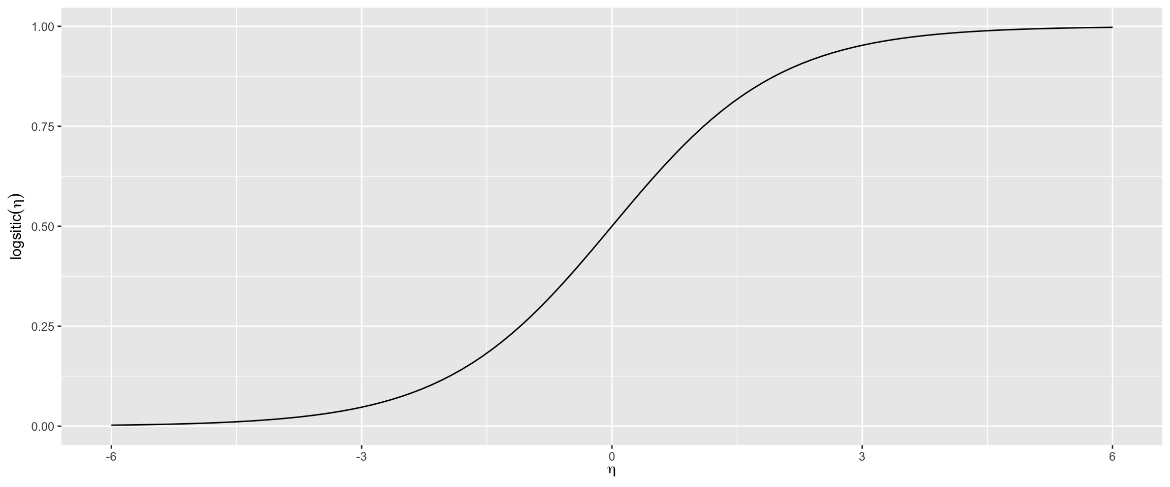
The logistic function is defined as:
Logistic function: \[logistic(\eta) = \frac{1}{1+exp^{-\eta}}\]
\[P(Y = 1 \vert X_i = x_i) = \frac{1}{1+exp^{-(\beta_0 + \beta_1X_1+ \dots \beta_n X_n)}}\]
where:
- \(\beta_n\) are the coeffcients we are searching
- \(X_n\) are the features
The second equation reads: The probability of \(Y=1\) given the value \(X=x_i\) which is exactly the result needed for a classification problem.
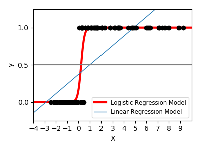
9.2.1 Python example logistic regression
An example of scikit-learn is given at https://scikit-learn.org/stable/auto_examples/linear_model/plot_logistic.html#sphx-glr-auto-examples-linear-model-plot-logistic-py and emphasises on the difference between linear and logistic regression. The synthetic data set has values either 0 or 1. This can be modeled quite well with logisitc regression, but not at all with linear regression.
The python code is given below
import numpy as np
import matplotlib.pyplot as plt

from sklearn import linear_model
from scipy.special import expit

# General a toy dataset:s it's just a straight line with some Gaussian noise:
xmin, xmax = -5, 5
n_samples = 100
np.random.seed(0)
X = np.random.normal(size=n_samples)
y = (X > 0).astype(np.float)
X[X > 0] *= 4
X += .3 * np.random.normal(size=n_samples)

X = X[:, np.newaxis]

# Fit the classifier
clf = linear_model.LogisticRegression(C=1e5)
clf.fit(X, y)

# and plot the result
plt.figure(1, figsize=(4, 3))
plt.clf()
plt.scatter(X.ravel(), y, color='black', zorder=20)
X_test = np.linspace(-5, 10, 300)

loss = expit(X_test * clf.coef_ + clf.intercept_).ravel()
plt.plot(X_test, loss, color='red', linewidth=3)

ols = linear_model.LinearRegression()
ols.fit(X, y)
plt.plot(X_test, ols.coef_ * X_test + ols.intercept_, linewidth=1)
plt.axhline(.5, color='.5')

plt.ylabel('y')
plt.xlabel('X')
plt.xticks(range(-5, 10))
plt.yticks([0, 0.5, 1])
plt.ylim(-.25, 1.25)
plt.xlim(-4, 10)
plt.legend(('Logistic Regression Model', 'Linear Regression Model'),
           loc="lower right", fontsize='small')
plt.tight_layout()
plt.show()