9.4 Support Vector Machine (SVM) TBD

A good explanation of the theory behind SVMs is given in (Tibshirani et al. 2013)

The support vector machine (SVM) is an extension of the support vector classifier that results from enlarging the feature space in a specific way, using kernels. We will now discuss this extension, the details of which are somewhat complex and are beyond the scope of this report. The main idea is to enlarge the feature space in order to accommodate a non-linear boundary between the classes. The kernel approach that we describe here is simply an efficient computational approach for enacting this idea.

9.4.1 Kernels

9.4.1.1 Polynomial Kernel

9.4.1.2 Radial Kernel

9.4.2 Python example for SVM

Two examples are given, both take images and classify them.

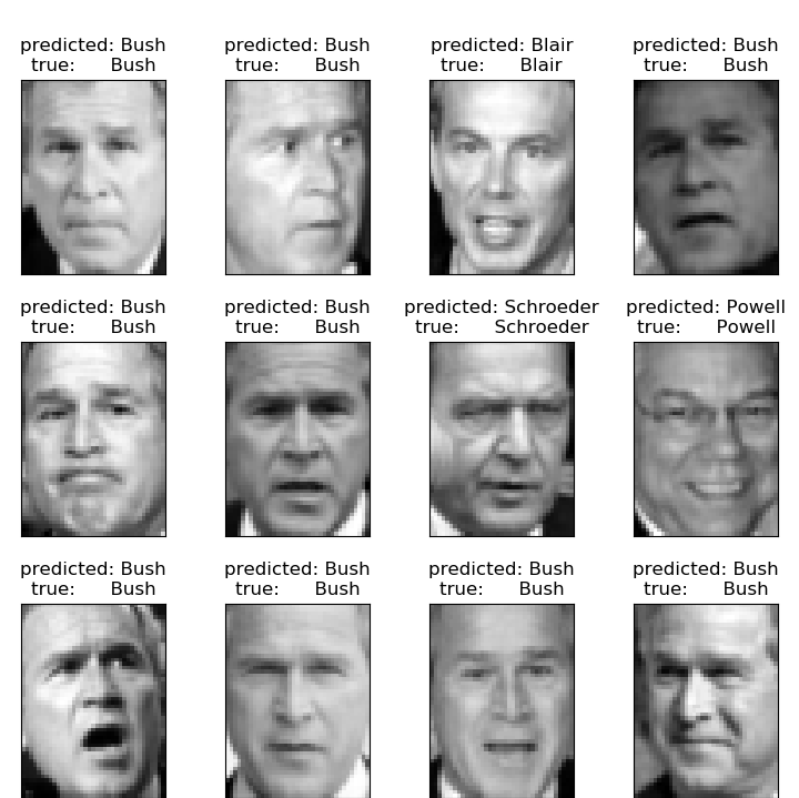
9.4.2.1 SVM face recognition

The following example is given at scikit-learn.org

It uses a SVM with

• rbf kernel
• grid search for hyper parameter
  • C
  • gamma
  • using scikit-learn GridSearchCV
• PCA to create input features
  • 150 dimensions

See below some examples of the resulting classification of the algorithm

Total dataset size:
n_samples: 1288
n_features: 1850
n_classes: 7
Extracting the top 150 eigenfaces from 966 faces
done in 0.320s
Projecting the input data on the eigenfaces orthonormal basis
done in 0.013s
Fitting the classifier to the training set
done in 28.379s
Best estimator found by grid search:
SVC(C=1000.0, break_ties=False, cache_size=200, class_weight='balanced',
    coef0=0.0, decision_function_shape='ovr', degree=3, gamma=0.005,
    kernel='rbf', max_iter=-1, probability=False, random_state=None,
    shrinking=True, tol=0.001, verbose=False)
Predicting people's names on the test set
done in 0.045s
                   precision    recall  f1-score   support

     Ariel Sharon       0.88      0.54      0.67        13
     Colin Powell       0.80      0.87      0.83        60
  Donald Rumsfeld       0.94      0.63      0.76        27
    George W Bush       0.83      0.98      0.90       146
Gerhard Schroeder       0.91      0.80      0.85        25
      Hugo Chavez       1.00      0.53      0.70        15
       Tony Blair       0.96      0.75      0.84        36

         accuracy                           0.85       322
        macro avg       0.90      0.73      0.79       322
     weighted avg       0.86      0.85      0.84       322


Confusion matrix

[[  7   1   0   5   0   0   0]
 [  1  52   0   7   0   0   0]
 [  0   3  17   7   0   0   0]
 [  0   3   0 143   0   0   0]
 [  0   1   0   3  20   0   1]
 [  0   4   0   2   1   8   0]
 [  0   1   1   6   1   0  27]]

The python code is given below

from time import time
import logging
import matplotlib.pyplot as plt

from sklearn.model_selection import train_test_split
from sklearn.model_selection import GridSearchCV
from sklearn.datasets import fetch_lfw_people
from sklearn.metrics import classification_report
from sklearn.metrics import confusion_matrix
from sklearn.decomposition import PCA
from sklearn.svm import SVC


print(__doc__)

# Display progress logs on stdout
logging.basicConfig(level=logging.INFO, format='%(asctime)s %(message)s')


# #############################################################################
# Download the data, if not already on disk and load it as numpy arrays

lfw_people = fetch_lfw_people(min_faces_per_person=70, resize=0.4)

# introspect the images arrays to find the shapes (for plotting)
n_samples, h, w = lfw_people.images.shape

# for machine learning we use the 2 data directly (as relative pixel
# positions info is ignored by this model)
X = lfw_people.data
n_features = X.shape[1]

# the label to predict is the id of the person
y = lfw_people.target
target_names = lfw_people.target_names
n_classes = target_names.shape[0]

print("Total dataset size:")
print("n_samples: %d" % n_samples)
print("n_features: %d" % n_features)
print("n_classes: %d" % n_classes)


# #############################################################################
# Split into a training set and a test set using a stratified k fold

# split into a training and testing set
X_train, X_test, y_train, y_test = train_test_split(
    X, y, test_size=0.25, random_state=42)


# #############################################################################
# Compute a PCA (eigenfaces) on the face dataset (treated as unlabeled
# dataset): unsupervised feature extraction / dimensionality reduction
n_components = 150

print("Extracting the top %d eigenfaces from %d faces"
      % (n_components, X_train.shape[0]))
t0 = time()
pca = PCA(n_components=n_components, svd_solver='randomized',
          whiten=True).fit(X_train)
print("done in %0.3fs" % (time() - t0))

eigenfaces = pca.components_.reshape((n_components, h, w))

print("Projecting the input data on the eigenfaces orthonormal basis")
t0 = time()
X_train_pca = pca.transform(X_train)
X_test_pca = pca.transform(X_test)
print("done in %0.3fs" % (time() - t0))


# #############################################################################
# Train a SVM classification model

print("Fitting the classifier to the training set")
t0 = time()
param_grid = {'C': [1e3, 5e3, 1e4, 5e4, 1e5],
              'gamma': [0.0001, 0.0005, 0.001, 0.005, 0.01, 0.1], }
clf = GridSearchCV(
    SVC(kernel='rbf', class_weight='balanced'), param_grid
)
clf = clf.fit(X_train_pca, y_train)
print("done in %0.3fs" % (time() - t0))
print("Best estimator found by grid search:")
print(clf.best_estimator_)


# #############################################################################
# Quantitative evaluation of the model quality on the test set

print("Predicting people's names on the test set")
t0 = time()
y_pred = clf.predict(X_test_pca)
print("done in %0.3fs" % (time() - t0))

print(classification_report(y_test, y_pred, target_names=target_names))
print(confusion_matrix(y_test, y_pred, labels=range(n_classes)))


# #############################################################################
# Qualitative evaluation of the predictions using matplotlib

def plot_gallery(images, titles, h, w, n_row=3, n_col=4):
    """Helper function to plot a gallery of portraits"""
    plt.figure(figsize=(1.8 * n_col, 2.4 * n_row))
    plt.subplots_adjust(bottom=0, left=.01, right=.99, top=.90, hspace=.35)
    for i in range(n_row * n_col):
        plt.subplot(n_row, n_col, i + 1)
        plt.imshow(images[i].reshape((h, w)), cmap=plt.cm.gray)
        plt.title(titles[i], size=12)
        plt.xticks(())
        plt.yticks(())


# plot the result of the prediction on a portion of the test set

def title(y_pred, y_test, target_names, i):
    pred_name = target_names[y_pred[i]].rsplit(' ', 1)[-1]
    true_name = target_names[y_test[i]].rsplit(' ', 1)[-1]
    return 'predicted: %s\ntrue:      %s' % (pred_name, true_name)

prediction_titles = [title(y_pred, y_test, target_names, i)
                     for i in range(y_pred.shape[0])]

plot_gallery(X_test, prediction_titles, h, w)

# plot the gallery of the most significative eigenfaces

eigenface_titles = ["eigenface %d" % i for i in range(eigenfaces.shape[0])]
plot_gallery(eigenfaces, eigenface_titles, h, w)

plt.show()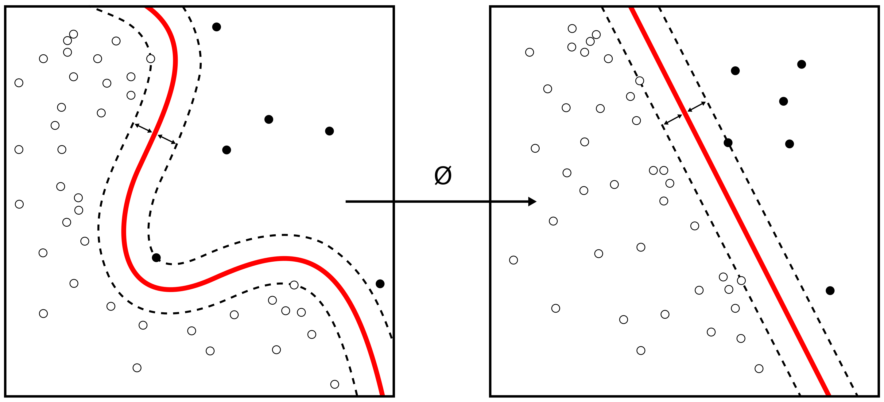

---

Figure from Alisneaky, svg version by User:Zirguezi [CC BY-SA (https://creativecommons.org/licenses/by-sa/4.0)]

9.4.2.2 SVM Image recognition

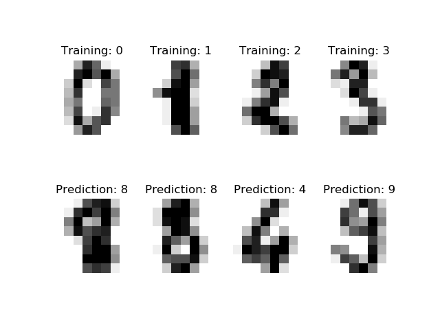
From the scikit-learn help page an example showing how the scikit-learn can be used to recognize images of hand-written digits.

The input data are hand written numbers

• Top: training data

• Bottom: Prediction

  

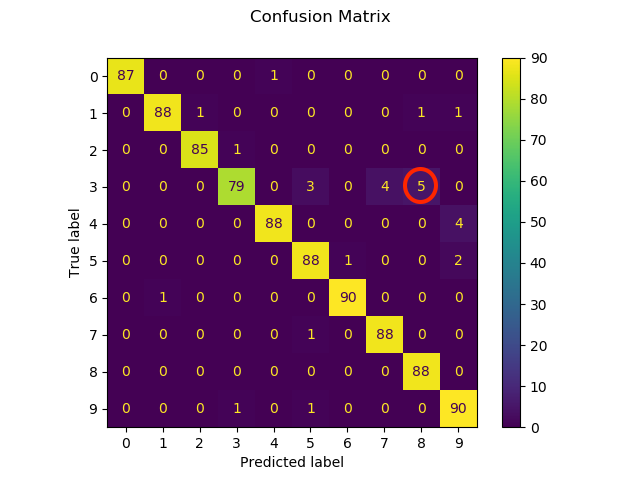
  The confusion matrix is given below and shows for example that a true “3” is often mistaken as a “8” (see red circle)

print(__doc__)

# Author: Gael Varoquaux <gael dot varoquaux at normalesup dot org>
# License: BSD 3 clause

# Standard scientific Python imports
import matplotlib.pyplot as plt

# Import datasets, classifiers and performance metrics
from sklearn import datasets, svm, metrics
from sklearn.model_selection import train_test_split

# The digits dataset
digits = datasets.load_digits()

# The data that we are interested in is made of 8x8 images of digits, let's
# have a look at the first 4 images, stored in the `images` attribute of the
# dataset.  If we were working from image files, we could load them using
# matplotlib.pyplot.imread.  Note that each image must have the same size. For these
# images, we know which digit they represent: it is given in the 'target' of
# the dataset.
_, axes = plt.subplots(2, 4)
images_and_labels = list(zip(digits.images, digits.target))
for ax, (image, label) in zip(axes[0, :], images_and_labels[:4]):
    ax.set_axis_off()
    ax.imshow(image, cmap=plt.cm.gray_r, interpolation='nearest')
    ax.set_title('Training: %i' % label)

# To apply a classifier on this data, we need to flatten the image, to
# turn the data in a (samples, feature) matrix:
n_samples = len(digits.images)
data = digits.images.reshape((n_samples, -1))

# Create a classifier: a support vector classifier
classifier = svm.SVC(gamma=0.001)

# Split data into train and test subsets
X_train, X_test, y_train, y_test = train_test_split(
    data, digits.target, test_size=0.5, shuffle=False)

# We learn the digits on the first half of the digits
classifier.fit(X_train, y_train)

# Now predict the value of the digit on the second half:
predicted = classifier.predict(X_test)

images_and_predictions = list(zip(digits.images[n_samples // 2:], predicted))
for ax, (image, prediction) in zip(axes[1, :], images_and_predictions[:4]):
    ax.set_axis_off()
    ax.imshow(image, cmap=plt.cm.gray_r, interpolation='nearest')
    ax.set_title('Prediction: %i' % prediction)

print("Classification report for classifier %s:\n%s\n"
      % (classifier, metrics.classification_report(y_test, predicted)))
disp = metrics.plot_confusion_matrix(classifier, X_test, y_test)
disp.figure_.suptitle("Confusion Matrix")
print("Confusion matrix:\n%s" % disp.confusion_matrix)

plt.show()

References

Tibshirani, Robert, G James, D Witten, and T Hastie. 2013. An Introduction to Statistical Learning-with Applications in r. New York, NY: Springer.