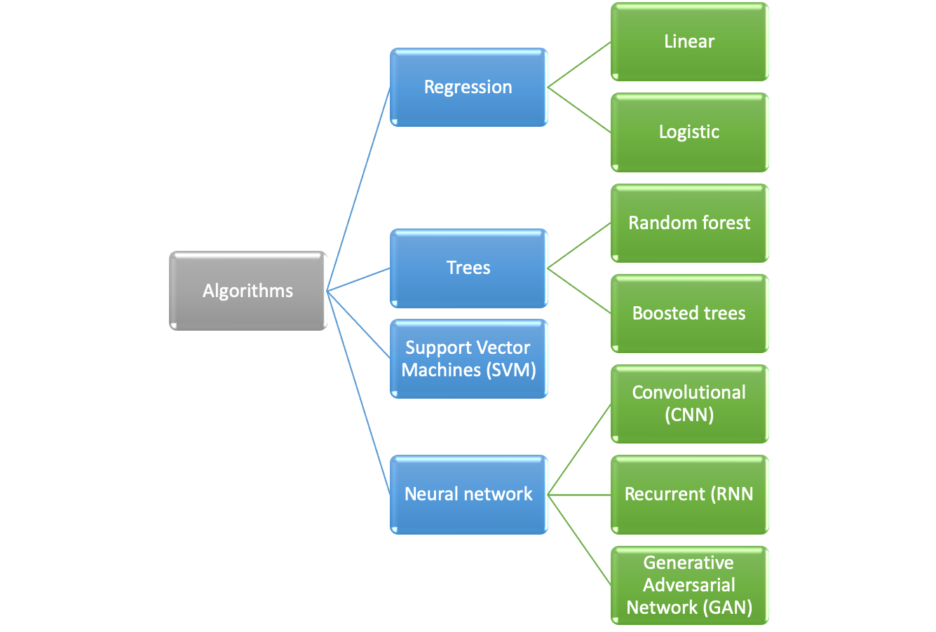
25.3 Algorithm selection
The following algorithms were meant to be investigated following the rule to start with the least complex one.
Determination which algorithm is best suited depends on:
Start with simplest algorithm to get a baseline
- doesn’t have to be a machine learning algorithm
Use simple algorithm for feature engineering
Use more complex algorithm if result is unsatisfactory
This is even more important since the algorithm was to be run on a satellite which where computing power is more limited than on earth
Start with simple model
25.3.1 Logistic regression
Logistic regression is the algorithm with the lowest computational complexity and therefore it was the algorithm with which the investigation for the suitable model would start
- Lowest computational complexity
- Start algorithm to determine suitable algorithm
- Details of algorithm are given in chapter 9.2
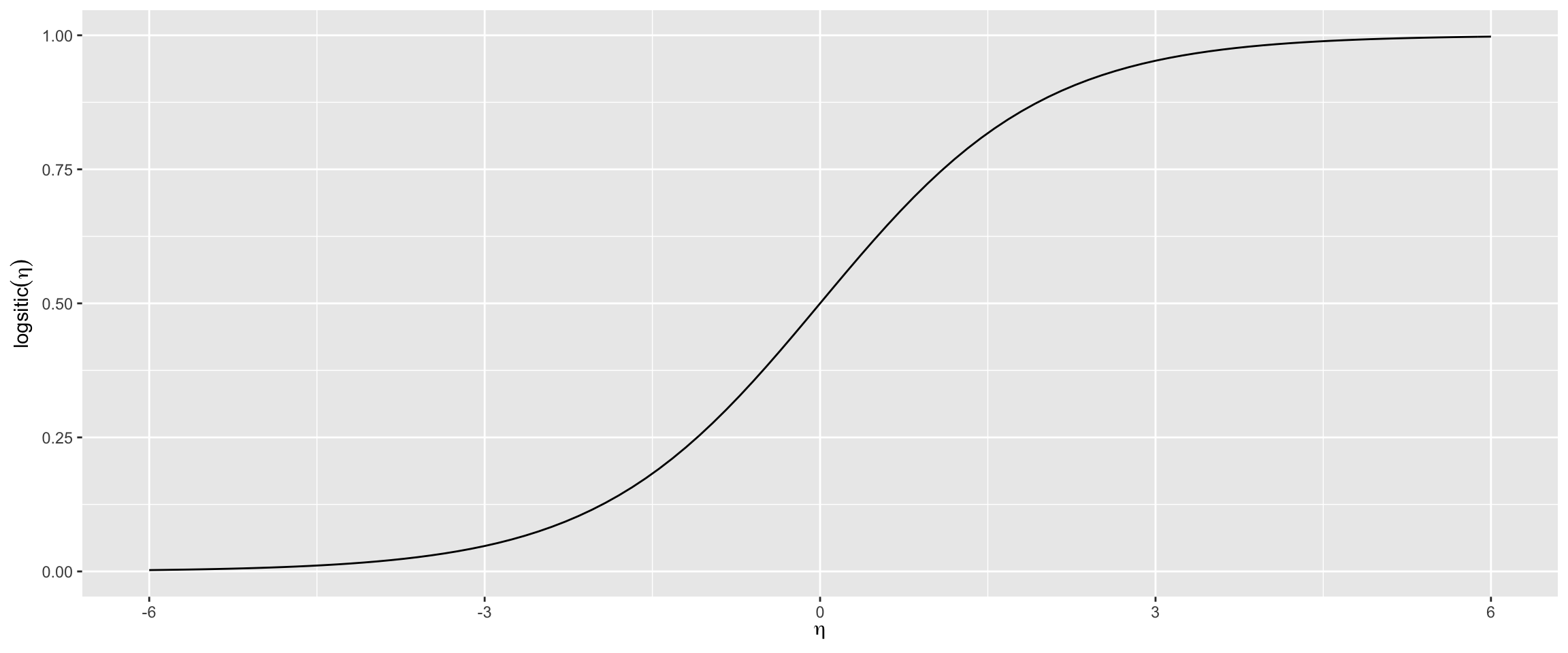
\[ logistic(\eta) = \frac{1}{1+exp^{-\eta}}\]
\[P(Y = 1 \vert X_i = x_i) = \frac{1}{1+exp^{-(\beta_0 + \beta_1X_1+ \dots \beta_n X_n)}}\]
where:
- \(\beta_n\) are the coeffcients we are searching
- \(X_n\) are the features
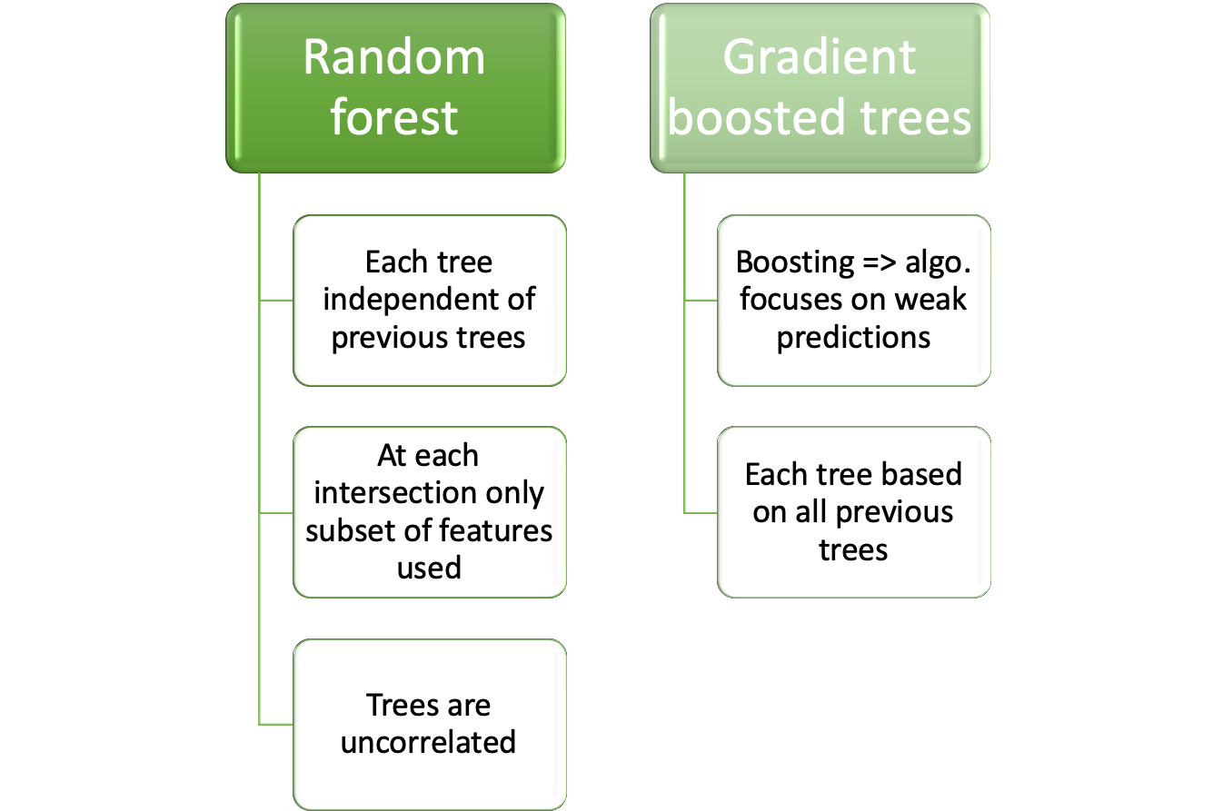
25.3.2 Tree based
Two dominant concepts are used for tree based algorithms:
Details on the algorithms are given at:
25.3.3 Support Vector Machine (SVM) TBD
- Support vector machine in chapter 9.4
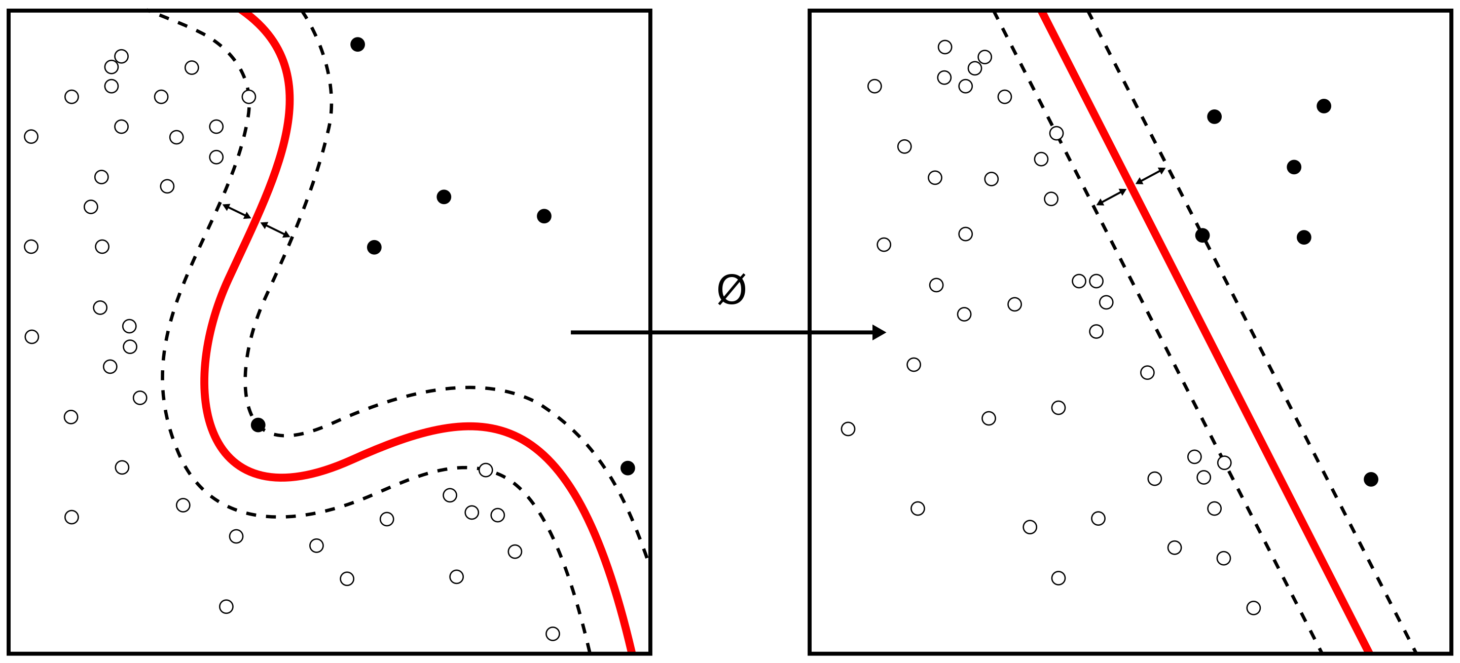
Figure from Alisneaky, svg version by User:Zirguezi [CC BY-SA (https://creativecommons.org/licenses/by-sa/4.0)]
Constrained optimization problem
\[\max_{\\beta_{1}, \ldots, \beta_{p}} M\]
\[\textrm{subject to} \sum_{j=1}^{p} \beta_{j}^{2}=1\]
\[y_{i}\left(\beta_{0}+\beta_{1} x_{i 1}+\ldots+\beta_{p} x_{i p}\right) \geq M\] for all i=1, \(\ldots\), N.